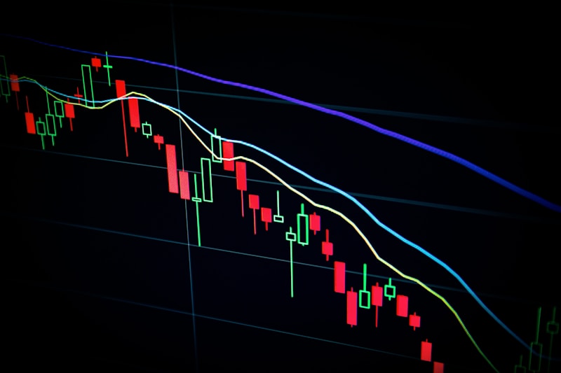
Algorithmic Trading 101: From Strategy to Execution
On a typical trading day in 2026, more than 70% of US equity volume is executed by computers running algorithms. No human types the order. No trader clicks “buy.” A Python script, a C++ engine, or a FPGA circuit decides what to trade, when to trade, and how much to trade, within microseconds of market signals. The trading floors filled with shouting humans in colorful jackets are gone; what remains are data centers, fiber optic cables, and server racks humming in upstate New Jersey.
Algorithmic trading is not a single thing. It is a spectrum from simple VWAP execution bots used by every pension fund, to medium-frequency statistical arbitrage, to ultra-low-latency market making that measures success in nanoseconds. What unifies the field is that the decisions are rules-based, systematic, and executed by software rather than discretion.
This article covers the full pipeline: designing a trading strategy, backtesting it, understanding execution algorithms, the role of HFT and market making, and the practical pitfalls that kill algorithms in production. It is the article that ties together everything you have learned about Python, options, SQL, statistics, and linear algebra into one coherent picture of modern electronic trading.
The guy in the colorful jacket shouting on the NYSE floor is now a Python script running in Equinix NY4. The job is the same. The method is not.
What Is Algorithmic Trading?
Algorithmic trading is the use of computer programs to make trading decisions and execute trades. An algorithm specifies:
- What to trade (which asset, which direction, what size)
- When to trade (entry and exit conditions based on market signals)
- How to trade (execution style: aggressive, passive, VWAP, etc.)
The spectrum is wide:
| Timeframe | Style | Examples |
|---|---|---|
| Microseconds | HFT, market making | Citadel Securities, Virtu, Jump |
| Seconds to minutes | Statistical arbitrage | Stat arb desks, XTX Markets |
| Minutes to hours | Intraday momentum, execution | Execution algos, some prop |
| Days to weeks | Trend following, mean reversion | CTAs (AHL, Winton, Man) |
| Weeks to months | Factor investing, systematic hedge funds | AQR, BlackRock, quant funds |
| Months to years | Long-term quantitative value | Renaissance, DE Shaw (some strategies) |
Why Algorithmic Trading Dominates
- Speed: computers react in microseconds; humans in seconds
- Scale: one algorithm can monitor thousands of symbols simultaneously
- Consistency: no fatigue, no emotion, no mistakes from boredom
- Backtestability: strategies can be tested on historical data before risking money
- Cost: electronic execution is orders of magnitude cheaper than human traders
- Market making: provides liquidity 24/7 with tight spreads
What Algorithms Cannot Do Well
- Understand narrative risk: a tweet, geopolitical event, or regime change
- Trade markets without enough data: small caps, illiquid names
- Handle truly novel situations: a crisis no algorithm was trained on
- Apply qualitative judgment: “this earnings call sounds bad” is not a feature
Key Insight: The “algorithmic vs discretionary” debate is mostly dead. Modern trading is a hybrid: algorithms handle execution, signal generation, and risk management; humans handle strategy design, model validation, and intervention during regime changes. The best firms combine both skills, not just one.
The stereotype of the yelling floor trader is 30 years dead. Walking through a modern trading floor is like walking through a data center with fewer humans and more Bloomberg terminals.
The Trading Strategy Lifecycle
Every systematic strategy goes through five stages:
1. Idea Generation
A strategy starts with a hypothesis about market behavior:
- “Stocks that drop 5% in a day tend to bounce back the next day”
- “When Fed statements are hawkish, long-dated Treasuries underperform”
- “Pairs of correlated stocks revert to their long-run spread”
Ideas come from reading academic papers, observing markets, analyzing data, or talking to other traders.
2. Research and Validation
Turn the hypothesis into a testable rule. Pull the historical data. Compute the signal. Measure how it would have performed.
3. Backtesting
Simulate the strategy on historical data. Calculate returns, volatility, Sharpe ratio, maximum drawdown, and turnover. Check robustness across periods and parameters.
4. Execution
Build the actual trading system. Connect to brokers, market data feeds, and risk systems. Handle orders, partial fills, errors, and edge cases.
5. Monitoring and Iteration
Once live, monitor the strategy’s performance vs. the backtest. Investigate deviations. Retire, retune, or enhance the strategy as market conditions evolve.
Most strategies fail at step 4 or 5. The difference between a cool backtest and a profitable live strategy is where careers are made and broken.
Strategy Archetypes
Most algorithmic strategies fall into a handful of recognizable categories.
1. Trend Following
Buy what is going up; sell what is going down. The cleanest implementation: if the 50-day moving average is above the 200-day, go long. When it crosses below, go short or exit.
Examples: CTAs (Commodity Trading Advisors) like Winton, AHL, Aspect.
Pros: Simple, well-documented, uncorrelated with equities during trends.
Cons: Suffers in sideways markets, whipsaw losses.
2. Mean Reversion
Bet that prices will revert to a long-run average. Trade against short-term moves.
Examples:
- Pairs trading: two correlated stocks diverge, expect them to converge
- Short-term equity reversal: a stock drops 5% in one day, buy it for the bounce
Pros: Works in ranging markets, usually high Sharpe ratio.
Cons: Catastrophic in crashes (mean reversion fails during regime changes).
3. Statistical Arbitrage
Multi-asset mean reversion using factor models. Identify pairs or baskets that should co-move, trade deviations from the expected relationship.
Examples: Renaissance Medallion Fund (the most successful hedge fund of all time), D.E. Shaw, Two Sigma.
Pros: Consistent, can be run at large scale.
Cons: Crowded trades get arbitraged away, requires very strong infrastructure.
4. Market Making
Post both bids and offers in a security, profit from the spread.
Examples: Citadel Securities, Virtu Financial, Jump Trading.
Pros: Huge returns on capital, low tail risk.
Cons: Requires ultra-low latency infrastructure, intense competition, short half-life of strategies.
5. Momentum
Longer-horizon version of trend following. Academic research (Jegadeesh and Titman, 1993) showed stocks with recent strong returns tend to continue outperforming for 3-12 months.
Examples: AQR, DFA factor funds.
Pros: Well-documented factor premium, long historical record.
Cons: Crashes badly at turning points (March 2009, November 2020).
6. Execution Algorithms
Not predictive strategies, but tools for efficiently executing large orders with minimal market impact. We cover these in detail below.
Backtesting: Where Strategies Go to Die
Backtesting is the process of simulating a strategy on historical data. Done well, it is the most important step in systematic trading. Done badly, it is the source of every failed quant fund in history.
A Basic Backtest in Python
import numpy as np
import pandas as pd
import yfinance as yf

# Download data
data = yf.download("SPY", start="2010-01-01", end="2026-01-01")["Close"]

# Moving average strategy: long when 50-day MA > 200-day MA
ma_short = data.rolling(50).mean()
ma_long = data.rolling(200).mean()

signal = (ma_short > ma_long).astype(int)
signal = signal.shift(1)  # Use yesterday's signal to avoid lookahead bias

# Daily returns
returns = data.pct_change()

# Strategy returns
strategy_returns = signal * returns

# Performance metrics
total_return = (1 + strategy_returns).prod() - 1
annual_return = (1 + total_return) ** (252 / len(returns)) - 1
annual_vol = strategy_returns.std() * np.sqrt(252)
sharpe = annual_return / annual_vol

print(f"Total return: {total_return:.2%}")
print(f"Annual return: {annual_return:.2%}")
print(f"Annual vol: {annual_vol:.2%}")
print(f"Sharpe: {sharpe:.2f}")

# Max drawdown
cumulative = (1 + strategy_returns).cumprod()
running_max = cumulative.cummax()
drawdown = (cumulative - running_max) / running_max
max_drawdown = drawdown.min()
print(f"Max drawdown: {max_drawdown:.2%}")
Critical Metrics
| Metric | Definition | What’s “Good” |
|---|---|---|
| Sharpe ratio | (Return - RF) / Volatility | >1 is decent, >2 is great, >3 is suspicious |
| Max drawdown | Worst peak-to-trough loss | Depends on strategy type |
| Calmar ratio | Annual return / max drawdown | >1 is strong |
| Sortino ratio | Return / downside vol | Better than Sharpe for skewed strategies |
| Turnover | Annual volume / capital | Affects transaction costs |
| Win rate | % of profitable trades | Context-dependent |
| Profit factor | Gross profit / gross loss | >1 by definition; higher is better |
The Most Dangerous Biases
1. Lookahead bias. Using information in the backtest that would not have been available at the time. Example: using the closing price to decide whether to have bought at the open. Always use shift(1) on signals.
2. Survivorship bias. Using today’s index constituents to backtest a strategy. Delisted companies are excluded, making the universe look rosier than it was. Use historical point-in-time universe data.
3. Overfitting. Trying thousands of parameter combinations until one produces a beautiful backtest. Such strategies rarely work out of sample. Use cross-validation and a held-out test period.
4. Data snooping. Seeing a pattern in data and “discovering” a strategy that captures it. Also known as “p-hacking.” The more hypotheses you test, the more likely you find spurious patterns.
5. Ignoring transaction costs. Including only direct commissions, not spread, market impact, or slippage. A strategy that looks great without costs can be unprofitable with them.
6. Ignoring borrow costs. Short positions require borrowing shares, which costs money and can be recalled at the worst time.
Key Insight: A good backtest is a sanity check, not a profit guarantee. If your strategy works in backtesting but fails in live trading, the usual culprits are transaction costs, impact, and parameter overfitting. Assume the real world is harsher than your simulation. It always is.
“Past performance does not guarantee future results” is the warning label every quant prospectus carries. It is legally required because it is scientifically true.
Execution Algorithms
Once a strategy decides to trade, how it trades matters enormously. Dropping a 1,000,000-share order into the market in one second would crash the price. Execution algorithms are designed to minimize market impact, the price degradation caused by your own trading.
VWAP (Volume-Weighted Average Price)
Split a large order into pieces proportional to the market’s historical volume profile throughout the day.
- Markets trade more volume at open and close, less at lunch
- VWAP places more of your order during high-volume periods
- Goal: execute at the volume-weighted average price
# Simplified VWAP schedule for a 100,000 share order
volume_profile = np.array([0.08, 0.05, 0.04, 0.03, 0.03, 0.04, 0.06, 0.10, 0.15])
# 9:30-10:00, 10-10:30, ..., 15:30-16:00

total_order = 100_000
slice_sizes = volume_profile * total_order
print("VWAP slices:", slice_sizes.astype(int))
TWAP (Time-Weighted Average Price)
Split the order evenly across time. Dumber than VWAP but predictable and simple.
- 10:00-10:05: 1,000 shares
- 10:05-10:10: 1,000 shares
- … (same rate all day)
Useful when you expect volume to be non-standard or want to avoid gaming by predators.
POV (Percentage of Volume)
Maintain your order at a fixed percentage of the market’s realized volume.
- If the market is trading 1M shares per minute, and you are set to 10% POV, you submit 100,000 shares that minute
- Adjust dynamically as market volume changes
Implementation Shortfall
Optimize the trade-off between market impact (trading too fast) and timing risk (trading too slow, market moves against you).
Tries to minimize deviation from the arrival price (price when the order was received).
Iceberg Orders
Display only a small portion of the order (“tip of the iceberg”); the rest stays hidden. As the visible portion fills, replenish from the hidden quantity.
Aggressive vs Passive
- Aggressive: cross the spread (market orders), pay for immediate execution
- Passive: join the bid/ask (limit orders), earn the spread but risk not filling
Most execution algos blend both based on urgency and market conditions.
High-Frequency Trading (HFT)
HFT is a subset of algorithmic trading focused on sub-millisecond decisions. Firms invest enormously in speed because the first order at a quote gets filled and the rest get nothing.
What HFT Firms Do
- Market making: post bid/ask quotes, profit from spread
- Arbitrage: exploit price differences between venues (NYSE vs ARCA, equity vs futures, ETF vs underlying)
- Latency arbitrage: react to news microseconds faster than others
- Statistical arbitrage at short horizons: predict prices seconds ahead
The Speed Arms Race
- 2000s: milliseconds mattered
- 2010s: microseconds mattered
- 2020s: nanoseconds matter
HFT firms spend hundreds of millions on:
- Colocation: placing servers inside exchange data centers (NY4, LD4, TY3)
- Fiber optics: straightest cables between exchanges
- Microwave/laser links: faster than fiber through air
- FPGA hardware: custom silicon for order processing
- Co-located market data: feeds delivered in nanoseconds
The NYSE-to-Nasdaq round trip is about 130 microseconds via microwave, faster than fiber.
Is HFT Good or Bad?
Arguments for: tighter spreads, deeper liquidity, better price discovery, lower costs for retail investors.
Arguments against: phantom liquidity that disappears in stress, flash crashes, predatory strategies against slow traders, resources spent on rent-seeking rather than productive activity.
The reality is complicated. HFT has absolutely reduced spreads for retail investors. It has also been involved in several flash crashes (May 2010, August 2015, February 2018). Regulation has lagged the technology.
The 2010 Flash Crash
On May 6, 2010, the Dow Jones dropped 1,000 points in minutes, then recovered almost completely. One trigger was a large sell algorithm (reportedly a Waddell & Reed E-mini trade) that executed too fast; HFT liquidity then withdrew, amplifying the crash. It was the moment regulators realized algorithmic trading had become too fast to fully understand.
Market Microstructure: The Rules of the Game
Understanding market microstructure is essential for execution and HFT.
The Order Book
At any moment, each exchange has a list of buy orders (bids) and sell orders (asks) at different prices:
| Side | Price | Quantity |
|---|---|---|
| Ask | $148.22 | 500 |
| Ask | $148.21 | 200 |
| Ask | $148.20 | 1,000 |
| Bid | $148.19 | 800 |
| Bid | $148.18 | 400 |
| Bid | $148.17 | 1,200 |
The spread is the difference between the best bid and best ask ($0.01 in this case).
Order Types
- Market order: buy/sell immediately at the best available price
- Limit order: buy/sell only at a specified price or better
- Stop order: triggers a market order when a price is hit
- Stop-limit order: triggers a limit order when a price is hit
- Fill-or-kill: execute immediately and completely or cancel
- Post-only: add liquidity only (limit order that won’t cross the spread)
Market Makers vs Takers
- Makers post limit orders that sit in the book, providing liquidity
- Takers submit marketable orders that cross the spread, removing liquidity
Most exchanges charge takers and pay makers (make-taker pricing), subsidizing liquidity provision.
Tick Size and Lot Size
Tick size: minimum price increment (usually $0.01 in US equities).
Lot size: minimum tradable quantity (usually 1 share for most US stocks, 100 shares traditionally).
Risk Management
Risk management kills more trading algorithms than bad strategies. A good algo with bad risk management blows up. A mediocre algo with good risk management survives.
1. Position Limits
Never let any single position exceed a fixed percentage of capital.
2. Stop Losses
Predefined price levels at which to exit losing positions. Controversial in quant circles; some argue it hurts performance for mean-reverting strategies.
3. Max Drawdown Circuit Breakers
If the strategy loses more than X% from peak, halt trading and investigate.
4. Exposure Limits
Gross exposure, net exposure, sector exposure, factor exposure. Each dimension needs its own limits.
5. Kill Switches
A master switch that cancels all open orders and flattens all positions. Every production algo needs one.
6. Real-Time Monitoring
Alerts when the algo behaves unexpectedly: larger-than-expected orders, positions outside limits, P&L swings, latency spikes.
The Knight Capital Disaster
On August 1, 2012, Knight Capital deployed new software that contained an old, unused code flag. The flag accidentally reactivated a dormant code path that sent uncontrolled orders. In 45 minutes, the algorithm traded $7 billion worth of securities, generating a $460 million loss that bankrupted the firm.
The lesson: software changes need rigorous deployment controls, kill switches, and rate limiters. Speed and efficiency are worthless if you cannot stop the machine.
Infrastructure: The Unglamorous Side
Algorithmic trading requires an entire infrastructure stack:
- Market data feed: real-time quotes and trades from exchanges
- Order management system (OMS): routes orders to brokers/exchanges
- Execution management system (EMS): controls execution algorithms
- Risk engine: real-time position and limit checks
- Post-trade reconciliation: match executions vs expected
- Compliance: regulatory reporting, audit logs
- Analytics: P&L attribution, transaction cost analysis
Small firms use vendor solutions (Bloomberg EMSX, FactSet, SS&C). Large firms build their own.
A Minimal Python Backtesting Framework
class BacktestEngine:
    def __init__(self, data, initial_capital=100_000):
        self.data = data
        self.capital = initial_capital
        self.positions = {}  # ticker -> quantity
        self.history = []

    def run(self, strategy):
        for date, row in self.data.iterrows():
            orders = strategy.generate_orders(row, self.positions)
            for order in orders:
                self._execute_order(order, row)
            self._record_pnl(date, row)

    def _execute_order(self, order, row):
        ticker = order["ticker"]
        quantity = order["quantity"]
        price = row[ticker]
        cost = quantity * price

        # Simple cost model: 5 bps slippage
        slippage = 0.0005 * abs(cost)

        self.capital -= cost + slippage
        self.positions[ticker] = self.positions.get(ticker, 0) + quantity

    def _record_pnl(self, date, row):
        market_value = sum(
            qty * row[ticker]
            for ticker, qty in self.positions.items()
        )
        total = self.capital + market_value
        self.history.append({"date": date, "total": total})

    def performance(self):
        df = pd.DataFrame(self.history).set_index("date")
        returns = df["total"].pct_change().dropna()
        sharpe = returns.mean() / returns.std() * np.sqrt(252)
        return {"sharpe": sharpe, "final_value": df["total"].iloc[-1]}
This is the skeleton. Real systems add transaction costs, market impact models, leverage, short-selling constraints, portfolio-level risk, and thousands of edge cases.
Common Pitfalls
Backtesting on the wrong data. Adjusted prices vs unadjusted, survivorship bias in the universe, wrong time zones for fills. Every mistake here falsifies your results.
Ignoring transaction costs. Commissions are small, but spread and market impact can be enormous. A strategy that turns over 10 times a year needs to beat its cost hurdle, not just have a positive signal.
Overfitting parameters. Testing 1,000 parameter combinations gives you a beautiful in-sample backtest and probably a losing strategy live. Use walk-forward testing and out-of-sample validation.
Latency assumptions. Your backtest assumes instantaneous execution. Real fills happen 50-500 ms later, at different prices, often partial. HFT strategies live and die on latency assumptions.
Ignoring regime change. A strategy that worked for 10 years can fail overnight when the market regime changes (2008, 2020). Understand what environment your strategy depends on.
No kill switch. The Knight Capital story. Always have a way to stop everything instantly.
Running a strategy past its capacity. A small strategy that’s profitable might stop working when scaled 10x because you become the market. Know your capacity.
Focusing on Sharpe, ignoring tail risk. A strategy with Sharpe 3.0 that blows up every 5 years has average returns. The worst day matters more than the average day.
Wrapping Up
Algorithmic trading has absorbed almost all electronic execution in modern markets. Every asset manager, hedge fund, and proprietary trading firm uses algorithms for at least part of their workflow. The field combines signal generation, execution optimization, risk management, and software engineering into a single discipline.
The entry ticket is broad: Python or C++ skills, understanding of market microstructure, statistical rigor, and infrastructure knowledge. The retention bar is higher: avoiding overfitting, handling regime changes, managing risk, and operating production systems reliably.
Most retail traders never make money systematically. Many institutional strategies fail out of sample. The few strategies that do work are carefully designed, rigorously tested, defensively engineered, and continuously monitored. There are no shortcuts and no silver bullets.
Algorithmic trading is the field where you get paid to be a good engineer, good statistician, and good risk manager all at once. Skimp on any one, and the market will find out before your bonus does.
Cheat Sheet
Key Questions & Answers
What is algorithmic trading?
The use of computer programs to make and execute trading decisions based on rules, signals, and parameters. Covers everything from simple VWAP execution algos to HFT market makers operating in microseconds. More than 70% of US equity volume is algorithmic.
What is the difference between VWAP and TWAP?
Both split large orders into pieces to reduce market impact. VWAP (Volume-Weighted Average Price) sizes pieces according to the historical volume profile (more at open and close). TWAP (Time-Weighted Average Price) spreads pieces evenly across time. VWAP is the industry default; TWAP is simpler and used when volume is unpredictable.
Why do backtests often look better than live performance?
Multiple reasons: lookahead bias, survivorship bias, overfitting, ignored transaction costs, unrealistic assumptions about execution. A good backtest is a sanity check, not a profit guarantee. The rule of thumb: expect half the backtest Sharpe in live trading, and be grateful when it is more.
What is HFT and why does speed matter?
High-Frequency Trading is the subset of algorithmic trading operating in microseconds or faster. It dominates market making, latency arbitrage, and short-term statistical strategies. Speed matters because the first order to a venue gets filled; second place gets nothing. Firms spend hundreds of millions on colocation, fiber, and FPGAs for nanosecond advantages.
Key Concepts at a Glance
| Concept | Summary |
|---|---|
| Algorithmic trading | Rule-based, software-executed trading decisions |
| HFT | Sub-millisecond algorithmic trading |
| Market making | Posting bids and offers, earning the spread |
| Trend following | Buy strength, sell weakness |
| Mean reversion | Bet against short-term moves |
| Statistical arbitrage | Multi-asset mean reversion using factor models |
| Backtesting | Simulating strategies on historical data |
| Sharpe ratio | (Return - RF) / Volatility, key performance metric |
| Max drawdown | Worst peak-to-trough loss |
| Lookahead bias | Using future info in backtests, inflates results |
| Overfitting | Tuning parameters to past data, fails out of sample |
| VWAP | Volume-weighted execution algorithm |
| TWAP | Time-weighted execution algorithm |
| POV | Percentage of Volume execution algorithm |
| Iceberg | Hide most of the order size from the market |
| Maker/taker | Providing vs removing liquidity from the book |
| Market impact | Price degradation caused by your own trading |
| Colocation | Placing servers inside exchange data centers |
| Kill switch | Emergency stop for all orders and positions |
| OMS/EMS | Order/Execution Management Systems |
Sources & Further Reading
- Aldridge, I., High-Frequency Trading: A Practical Guide to Algorithmic Strategies, Wiley
- Chan, E.P., Algorithmic Trading: Winning Strategies and Their Rationale, Wiley
- Chan, E.P., Quantitative Trading: How to Build Your Own Algorithmic Trading Business, Wiley
- Johnson, B., Algorithmic Trading and DMA, 4Myeloma Press
- Hasbrouck, J., Empirical Market Microstructure, Oxford University Press
- Narang, R.K., Inside the Black Box: A Simple Guide to Quantitative and High-Frequency Trading, Wiley
- Lewis, M., Flash Boys: A Wall Street Revolt, W.W. Norton
- Jegadeesh, N. & Titman, S. (1993), Returns to Buying Winners and Selling Losers, Journal of Finance
- SEC & CFTC (2010), Findings Regarding the Market Events of May 6, 2010
- Kissell, R., The Science of Algorithmic Trading and Portfolio Management, Academic Press
- Harris, L., Trading and Exchanges: Market Microstructure for Practitioners, Oxford University Press
- Gould, M.D. et al. (2013), Limit Order Books, Quantitative Finance